M-ary Alphabet Codes – Hadamard Codes

This will likely be the most technical/mathy topic on this site. After discovering this family of codes, I wrote several python scripts to explore the topic more. Some time later, I wrote the following paper on the topic. However, I never submitted it for publication and it just collected dust. After launching this site, I decided to make the paper available for anyone who may have an interest in the topic. Scroll to the end of the document to see some of the code plots generated using the aforementioned python scripts.

Abstract

This page describes a general set of matrices that exhibit the same properties as
Hadamard Matrices and Binary Walsh Matrices. This general set of matrices works
with any alphabet size, not just an alphabet of 2 (binary). Python scripts for
generating these matrices can be found on GitHub[1].

Definitions/Conventions

The $\oplus$ operator denotes an exclusive-or.
The % operator denotes a modulo operation.
The $[\oplus]$ operator denotes a special operation referred to in this document as a “recursive exclusive-or”. Given two matrices, M and M with dimensions $(x_1,y_1)$
and $(x_2,y_2)$ , the recursive exclusive-or of the two matrices will result in a matrix of dimension $(x_1\times x_2,y_1\times y_2)$ , where each entry of M is exclusive-ored to a copy of M .

M_1 [\oplus] M_2 = \begin{bmatrix}{M_1(1,1) \oplus M_2} &{\ldots}&{M_1(x_1,1) \oplus M_2} \\{\vdots }&{\ddots}& {\vdots}\\ {M_1(1,y_1) \oplus M_2} & {\ldots} & {M_1(x_1,y_1) \oplus M_2} \end{bmatrix}

For example,

M_1 = \begin{bmatrix} 0 & 1\\ 1 & 0 \end{bmatrix}\enspace M_2 = \begin{bmatrix}1\\1\\0 \end{bmatrix} \\ M_1 [\oplus] M_2 = \begin{bmatrix}0\oplus\begin{bmatrix}1\\1\\0 \end{bmatrix} & 1\oplus\begin{bmatrix}1\\1\\0 \end{bmatrix} \\1\oplus \begin{bmatrix}1\\1\\0 \end{bmatrix} & 0\oplus \begin{bmatrix}1\\1\\0 \end{bmatrix} \end{bmatrix} = \begin{bmatrix} \begin{bmatrix}1\\1\\0 \end{bmatrix} \begin{bmatrix}0\\0\\1 \end{bmatrix}\\ \begin{bmatrix}0\\0\\1 \end{bmatrix} \begin{bmatrix}1\\1\\0 \end{bmatrix} \end{bmatrix} = \begin{bmatrix}1&0\\1&0\\0&1\\0&1\\0&1\\1&0 \end{bmatrix}

The $[\times]$ operator denotes a Kronecker Product[2]. Given two matrices, $M_1$ and $M_2$ with dimensions $(x_1,y_1)$ and $(x_2,y_2)$ , the Kronecker Product of the two matrices will result in a matrix of dimension $x_1\times x_2,y_1\times y_2$ , where each entry of $M_1$ is multiplied with a copy of $M_2$ .

M_1 [\times] M_2 = \begin{bmatrix}{M_1(1,1) \times M_2} &{\ldots}&{M_1(x_1,1) \times M_2} \\{\vdots }&{\ddots}& {\vdots}\\ {M_1(1,y_1) \times M_2} & {\ldots} & {M_1(x_1,y_1) \times M_2} \end{bmatrix}

For example,

M_1 = \begin{bmatrix} 2 & 3\\ 7 & 5 \end{bmatrix}\enspace M_2 = \begin{bmatrix}1\\6\\4 \end{bmatrix} \\ M_1 [\times] M_2 = \begin{bmatrix}2\times\begin{bmatrix}1\\6\\4 \end{bmatrix} & 3\times\begin{bmatrix}1\\6\\4 \end{bmatrix} \\7\times \begin{bmatrix}1\\6\\4 \end{bmatrix} & 5\times \begin{bmatrix}1\\6\\4 \end{bmatrix} \end{bmatrix} = \begin{bmatrix} \begin{bmatrix}2\\12\\8 \end{bmatrix} \begin{bmatrix}3\\18\\12 \end{bmatrix}\\ \begin{bmatrix}7\\42\\28 \end{bmatrix} \begin{bmatrix}5\\30\\20 \end{bmatrix} \end{bmatrix} = \begin{bmatrix}2&3\\12&18\\8&12\\7&5\\42&30\\28&20 \end{bmatrix}

The $[+]$ operator denotes a special operation referred to in this document as a “recursive sum”. Given two matrices, $M_1$ and $M_2$ with dimensions $(x_1,y_1)$ and $(x_2,y_2)$ , the recursive sum of the two matrices will result in a matrix of dimension $(x_1\times x_2,y_1\times y_2)$ , where each entry of $M_1$ is added to a copy of $M_2$ . In the definition below, J is a matrix of all ones with dimension $(x_2,y_2)$ , used to allow the addition of scalar entry from $M_1$ to the matrix $M_2$ . Note that this operation is not the same as a Kronecker Sum[3].

M_1 [+] M_2 = \begin{bmatrix}{M_1(1,1) J+ M_2} &{\ldots}&{M_1(x_1,1) J+ M_2} \\{\vdots }&{\ddots}& {\vdots}\\ {M_1(1,y_1) J+ M_2} & {\ldots} & {M_1(x_1,y_1) J+ M_2} \end{bmatrix}

For example,

M_1 = \begin{bmatrix} 2 & 3\\ 7 & 5 \end{bmatrix}\enspace M_2 = \begin{bmatrix}1\\6\\4 \end{bmatrix}

Since $M_2$ is a 1×3 matrix, J is defined as follows:

J =\begin{bmatrix}1\\1\\1\end{bmatrix}

M_1 [+] M_2 = \begin{bmatrix}2\times\begin{bmatrix}1\\1\\1\end{bmatrix}+\begin{bmatrix}1\\6\\4 \end{bmatrix} & 3\times\begin{bmatrix}1\\1\\1\end{bmatrix}+\begin{bmatrix}1\\6\\4 \end{bmatrix} \\7\times \begin{bmatrix}1\\1\\1\end{bmatrix}+\begin{bmatrix}1\\6\\4 \end{bmatrix} & 5\times \begin{bmatrix}1\\1\\1\end{bmatrix}+\begin{bmatrix}1\\6\\4 \end{bmatrix} \end{bmatrix} = \begin{bmatrix}\begin{bmatrix}2\\2\\2\end{bmatrix}+\begin{bmatrix}1\\6\\4 \end{bmatrix} & \begin{bmatrix}3\\3\\3\end{bmatrix}+\begin{bmatrix}1\\6\\4 \end{bmatrix} \\ \begin{bmatrix}7\\7\\7\end{bmatrix}+\begin{bmatrix}1\\6\\4 \end{bmatrix} & \begin{bmatrix}5\\5\\5\end{bmatrix}+\begin{bmatrix}1\\6\\4 \end{bmatrix} \end{bmatrix} = \begin{bmatrix}3&4\\8&9\\6&7\\8&6\\13&11\\11&9 \end{bmatrix}

Background

Hadamard Matrices and their cousins, Binary Walsh Matrices, are commonly used in digital communications and signal processing for their ability to produce orthogonal code sequences [4][5]. Hadamard matrices are comprised of the values 1 and -1, while Binary Walsh Matrices are comprised of the values 0 and 1. The two matrices are homomorphic and exhibit the following mapping [4]:

\big\{1,-1,\times,[\times]\big\} \leftrightarrow \big\{0,1,\oplus,[\oplus]\big\}

Both matrices are symmetrical so each matrix is also equal to the transverse of the matrix. That is:

H_{2^n} =H_{2^n}^T\\ W_{2^n} =W_{2^n}^T

The sum of every value in each column or row of a Hadamard Matrix, except for the first column and row, is zero. The sum of every value in each column or row of a Binary Walsh Matrix, except for the first column and row, is equal to half the height or width.

Sylvester’s construction can be used on both family of matrices to generate higher order matrices using lower order matrices [4]. This is shown as follows.

H_1 = [1]\\ H_2 = \begin{bmatrix}H_1&H_1\\H_1&-H_1\end{bmatrix} = \begin{bmatrix}1&1\\1&-1\end{bmatrix}\\ H_4 = \begin{bmatrix}H_2&H_2\\H_2&-H_2\end{bmatrix} = \begin{bmatrix}1&1&1&1\\1&-1&1&-1\\1&1&-1&-1\\1&-1&-1&1\end{bmatrix} \\ H_{2^n} = \begin{bmatrix}H_{2^{n-1}}&H_{2^{n-1}}\\H_{2^{n-1}}&-H_{2^{n-1}}\end{bmatrix} = H_2[\times]H_{2^{n-1}}

W_1 = [0]\\ W_2 = \begin{bmatrix}W_1&W_1\\W_1&\overline{W_1}\end{bmatrix} = \begin{bmatrix}0&0\\0&1\end{bmatrix} \\ W_4 = \begin{bmatrix}W_2&W_2\\W_2&\overline{W_2}\end{bmatrix} = \begin{bmatrix}0&0&0&0\\0&1&0&1\\0&0&1&1\\0&1&1&0\end{bmatrix} \\ W_{2^n} = \begin{bmatrix}W_{2^{n-1}}&W_{2^{n-1}}\\W_{2^{n-1}}&\overline{W_{2^{n-1}}}\end{bmatrix} = W_2[\oplus]W_{2^{n-1}}

For values of n that are greater than or equal to 2.

Hadamard matrices satisfy the following relationship, proving that they are
orthogonal [4].

H_{2^n}H_{2^n}^T = 2^nI_{2^n}

For example,

H_2=H_2^T = \begin{bmatrix}1&1\\1&-1\end{bmatrix}\\ H_2H_2^T = \begin{bmatrix}1&1\\1&-1\end{bmatrix}\begin{bmatrix} 1\times 1+ 1\times 1& 1\times 1+ 1\times -1\\ 1\times 1+ -1\times 1& 1\times 1+ -1\times -1\end{bmatrix} = \begin{bmatrix}2&0\\0&2\end{bmatrix} =2\begin{bmatrix}1&0\\0&1\end{bmatrix} = 2I_2

Observations

The homomorphic relationship between Hadamard Matrices and Binary Walsh Matrices can be can be be expressed simply if the values in each matrix are treated as vectors. The polar equivalent of the values 1 and -1 from Hadamard Matrices are $1\angle 0^\circ$ and $1\angle 180^\circ$ , respectively. From this, the following relationship can be made.

H_{2^n} = 1\angle180^\circ W_{2^n}

For example when n=1,

W_2 = \begin{bmatrix}0&0\\0&1\end{bmatrix}\\ H_2 = \begin{bmatrix}1&1\\1&-1\end{bmatrix} = 1\angle \begin{bmatrix}0^\circ&0^\circ\\0^\circ&180^\circ\end{bmatrix} = 1\angle180^\circ \begin{bmatrix}0&0\\0&1\end{bmatrix} = 1\angle 180^\circ W_2

Furthermore, multiplication of two vectors on the unit circle is equivalent to the sum of their angles. If the angles from both vectors are different (one $0^\circ$ and the other $180^\circ$ ), then the sum of the angles is $180^\circ$ . If the angles from both vectors are the same (both $0^\circ$ or both $180^\circ$ ), then the sum of the angles is $0^\circ$ (or $360^\circ$ which is equal to $0^\circ$ ). So this same relationship also translates the multiplications present in Sylvester’s construction of Hadamard Matrices into the exclusive-ors present in the construction of Binary Walsh Matrices.

Hadamard Matrices can be multiplied with the transverse matrix using vectors as well. This matrix multiplication is a dot product. The values in each matrix are angles on the unit circle, so the dot product of these values is the the cosine of the angle between the two vectors. This is shown as follows:

H_2T_2^T = 1\angle\begin{bmatrix}0^\circ&0^\circ\\0^\circ&180^\circ\end{bmatrix}1\angle\begin{bmatrix}0^\circ&0^\circ\\0^\circ&180^\circ\end{bmatrix}\\ = 1\angle\begin{bmatrix}cos(0^\circ)+cos(0^\circ)&cos(0^\circ)+cos(-180^\circ)\\cos(0^\circ)+cos(180^\circ)&cos(0^\circ)+cos(0^\circ)\end{bmatrix}\\ =\begin{bmatrix}2&0\\0&2\end{bmatrix} = 2\begin{bmatrix}1&0\\0&1\end{bmatrix} = 2I_2

m-ary Alphabet Matrices

Hadamard Matrices and Binary Walsh Matrices are binary matrices. A more general definition is required to support all alphabet lengths (m). This definition is as follows:

G_{m,1} = \begin{bmatrix}0 & \ldots &0 \\ \vdots & A_m \\0\end{bmatrix}

Where $G_{m,1}$ is an m by m matrix. The letter “G” stands for generalized and was chosen because it neighbors “H”.

G_{m,2} = \begin{bmatrix}G_{m,1}&\ldots & G_{m,1}\\ \vdots &\big(A_m[+]G_{m,1}\big)\%m\\G_{m,1}\end{bmatrix}

Where $G_{m,2}$ is a $m^2$ by $m^2$ matrix which can be factored as follows:

G_{m,2} = \big(G_{m,1}[+]G_{m,1}\big)\%m

Similarly,

G_{m,n} = \begin{bmatrix}G_{m,n-1}&\ldots & G_{m,n-1}\\ \vdots &\big(A_m[+]G_{m,n-1}\big)\%m\\G_{m,n-1}\end{bmatrix} = \big(G_{m,1}[+]G_{m,n-1}\big)\%m

Where $G_{m,n}$ is a $m^n$ by $m^n$ matrix.

G_{m,2}' = \big(G_{m,1}[+]G_{m,1}\big)\%m

In all cases m and n are each greater than or equal to 2. Also $A_m$ is an (m-1) by (m-1) matrix, defined as follows:

A_2 = [1] \\ A_3 = \big\{ \begin{bmatrix}1 & 2 \\ 2 & 1\end{bmatrix}, \begin{bmatrix}2&1\\1&2\end{bmatrix} \big\}\\ A_4 =\big\{ \begin{bmatrix}1&2&3\\2&3&1\\3&1&2\end{bmatrix}, \begin{bmatrix}2&3&1\\3&1&2\\1&2&3\end{bmatrix}, \begin{bmatrix}3&1&2\\1&2&3\\2&3&1\end{bmatrix}, \begin{bmatrix}1&3&2\\3&2&1\\2&1&3\end{bmatrix}, \begin{bmatrix}3&2&1\\2&1&3\\1&3&2\end{bmatrix}, \begin{bmatrix}2&1&3\\1&3&2\\3&2&1\end{bmatrix} \big\}\\ A_m = \big\{\begin{bmatrix} 1&2&\ldots&m-2& m-1\\ 2&3&\ldots & m-1 & 1\\ \vdots&\vdots&\ddots&\vdots&\vdots\\ m-2&m-1&\ldots&m-4&m-3\\ m-1&1&\ldots&m-3&m-2\end{bmatrix}, \ldots\big\}

Note that the number of possible A matrices for a given value of m is (m-1)!, of which there are (m-2) unique permutations, and (m-2)! rotations of each
permutation.

Finally, the matrices can be expressed in vector form as follows:

G_{m,n}' = 1\angle\frac{360^\circ}{m}G_{m,n}

The sum of vectors in each row and column, except the first row/column, is zero for every matrix $G_{m,n}$ . Also, all rows/columns are orthogonal and satisfy the following relation:

G_{m,n}'G_{m,n}'^T = m^n I_{m,n}

Where $I_{m,n}$ is a $m^n$ by $m^n$ identity matrix.

M-ary alphabet matrices appear to have some similarities with a couple low order Complex Hadamard Matrices[6]. However, the majority of the matrices are vastly different as are the methods of construction.

Examples

Example: m=2

This example will show that Hadamard Matrices and Binary Walsh matrices are special cases of m-ary alphabet matrices.

A_2 = [1]\\ G_{2,1} = \begin{bmatrix}0 & \ldots &0 \\ \vdots & A_2 \\0\end{bmatrix} = \begin{bmatrix}0 & 0\\0&1\end{bmatrix}

$G_{2,2}$ is constructed as follows:

G_{2,2} = \big(G_{2,1}[+]G_{2,1}\big)\%2 =\begin{bmatrix} 0\times \begin{bmatrix}1 & 1\\1&1\end{bmatrix}+\begin{bmatrix}0 & 0\\0&1\end{bmatrix} & 0\times \begin{bmatrix}1 & 1\\1&1\end{bmatrix}+\begin{bmatrix}0 & 0\\0&1\end{bmatrix}\\0\times \begin{bmatrix}1 & 1\\1&1\end{bmatrix}+\begin{bmatrix}0 & 0\\0&1\end{bmatrix}&1\times \begin{bmatrix}1 & 1\\1&1\end{bmatrix}+\begin{bmatrix}0 & 0\\0&1\end{bmatrix}\end{bmatrix} \%2= \begin{bmatrix}0&0&0&0\\0&1&0&1\\0&0&1&1\\0&1&1&0\end{bmatrix}

Note that $G_{2,1}=W_2$ and $G_{2,2}=W_4$ . The process can be repeated to show that the following is true for all positive values of n.

G_{2,n} = W_{2^n}

This allows the relationship $G_{2,n}' = H_{2^n}$ to be derived as follows:

G_{2,n}' = 1\angle \frac{360^\circ}{2}G_{2,n}=1\angle 180^\circ W_{2^n}=H_{2^n}

Therefore Hadamard Matrices and Binary Walsh Matrices are simply m-ary
Alphabet Matrices where m=2.

Example: m=3

This example will show how to construct higher order m-ary alphabet matrices for values of m other than 2. It will also show that that m-ary alphabet relationships described above hold also true for such values of m.

A_3 = \begin{bmatrix}1 & 2 \\ 2 & 1\end{bmatrix} or \begin{bmatrix}2&1\\1&2\end{bmatrix}

For this example, we will use the first matrix.

G_{3,1} = \begin{bmatrix}0 & \ldots &0 \\ \vdots & A_3 \\0\end{bmatrix} = \begin{bmatrix}0 & 0 &0\\0&1&2\\0&2&1\end{bmatrix}

$G_{3,2}$ is constructed as follows:

G_{3,2} = \big(G_{3,1}[+]G_{3,1}\big)\%3 =\begin{bmatrix} 0\times \begin{bmatrix}1&1&1\\1&1&1\\1&1&1\end{bmatrix}+ \begin{bmatrix}0&0&0\\0&1&2\\0&2&1\end{bmatrix}& 0\times \begin{bmatrix}1&1&1\\1&1&1\\1&1&1\end{bmatrix}+ \begin{bmatrix}0&0&0\\0&1&2\\0&2&1\end{bmatrix}& 0\times \begin{bmatrix}1&1&1\\1&1&1\\1&1&1\end{bmatrix}+ \begin{bmatrix}0&0&0\\0&1&2\\0&2&1\end{bmatrix}\\ 0\times \begin{bmatrix}1&1&1\\1&1&1\\1&1&1\end{bmatrix}+ \begin{bmatrix}0&0&0\\0&1&2\\0&2&1\end{bmatrix}& 1\times \begin{bmatrix}1&1&1\\1&1&1\\1&1&1\end{bmatrix}+ \begin{bmatrix}0&0&0\\0&1&2\\0&2&1\end{bmatrix}& 2\times \begin{bmatrix}1&1&1\\1&1&1\\1&1&1\end{bmatrix}+ \begin{bmatrix}0&0&0\\0&1&2\\0&2&1\end{bmatrix}\\ 0\times \begin{bmatrix}1&1&1\\1&1&1\\1&1&1\end{bmatrix}+ \begin{bmatrix}0&0&0\\0&1&2\\0&2&1\end{bmatrix}& 2\times \begin{bmatrix}1&1&1\\1&1&1\\1&1&1\end{bmatrix}+ \begin{bmatrix}0&0&0\\0&1&2\\0&2&1\end{bmatrix}& 1\times \begin{bmatrix}1&1&1\\1&1&1\\1&1&1\end{bmatrix}+ \begin{bmatrix}0&0&0\\0&1&2\\0&2&1\end{bmatrix}\end{bmatrix} \%3 \\ = \begin{bmatrix} 0&0&0&& 0&0&0&& 0&0&0\\ 0&1&2&& 0&1&2&& 0&1&2\\ 0&2&1&& 0&2&1&& 0&2&1\\ \\ 0&0&0&& 1&1&1&& 2&2&2\\ 0&1&2&& 1&2&0&& 2&0&1\\ 0&2&1&& 1&0&2&& 2&1&0\\ \\ 0&0&0&& 2&2&2&& 1&1&1\\ 0&1&2&& 2&0&1&& 1&2&0\\ 0&2&1&& 2&1&0&& 1&0&2 \end{bmatrix}

The relationship $G_{m,n}'G_{m,n}'^T$ will now be demonstrated using $G_{3,1}'$ . This matrix was chosen because larger matrices would consume considerably more space.

G_{3,1}' = 1\angle\frac{360}{3}\begin{bmatrix}0&0&0\\0&1&2\\0&2&1\end{bmatrix} = 1\angle\begin{bmatrix}0^\circ&0^\circ&0^\circ\\0^\circ&120^\circ&240^\circ\\0^\circ&240^\circ&120^\circ\end{bmatrix}

Multiplication of $G_{3,1}'$ with $G_{3,1}'^T$ results in the dot product of the two matrices. The values in each matrix are angles on the unit circle, so the dot product of these values is the the cosine of the angle between the two vectors. This is shown as follows:

G_{3,1}'G_{3,1}'^T =\begin{bmatrix} \big(cos(0^\circ)+cos(0^\circ)+cos(0^\circ)\big)& \big(cos(0^\circ)+cos(-120^\circ)+cos(-240^\circ)\big)& \big(cos(0^\circ)+cos(-240^\circ)+cos(-120^\circ)\big)\\ \big(cos(0^\circ)+cos(120^\circ)+cos(240^\circ)\big)& \big(cos(0^\circ)+cos(0^\circ)+cos(0^\circ)\big)& \big(cos(0^\circ)+cos(-120^\circ)+cos(120^\circ)\big)\\ \big(cos(0^\circ)+cos(240^\circ)+cos(120^\circ)\big)& \big(cos(0^\circ)+cos(120^\circ)+cos(-120^\circ)\big)& \big(cos(0^\circ)+cos(0^\circ)+cos(0^\circ)\big) \end{bmatrix}\\ =\begin{bmatrix}3&0&0\\0&3&0\\0&0&3\end{bmatrix} = 3I_{3,1}

References

[1] nary-codes on GitHub
[2] Kronecker Product Wikipedia Article
[3] Kronecker Sum Wikipedia Article
[4] Hadamard Matrix Wikipedia Article
[5] Walsh Matrix Wikipedia Article
[6] Complex Hadamard Matrix Wikipedia Article

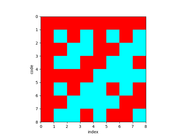
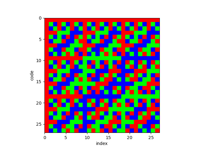
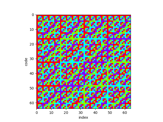
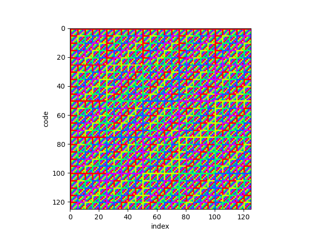
Bonus Content

Below are some images created using the the plot_matrix.py script found on GitHub. Each image shows the effect of increasing the code alphabet (m), while keeping the code order (n) the same. The dimensions of each matrix are $m^n$ . In these plots the code order (n) was set to 3.